
In many situations a lot of time and money are spent to develop a SQL Server data warehouse solution only to have the resulting queries perform poorly at execution time. This can be a very frustrating situation for both IT, those responsible for maintaining the system, and the business, those who are consuming the data produced by the data warehouse system.
However, as painful as poor query performance is for the end user, in most cases it is only a symptom of a much larger SQL Server Data Warehouse architectural problem. In many cases the even basic performance capabilities such as throughput (MB) are unknown. Without knowing the base line performance of how the hardware preforms with a data warehouse specific workload it is impossible to ever know how to performance tune it.
However if you do know the throughput (MB/second) of the data warehouse server then all that you need to do is to compare that to amount of data that is being returned by each query to get and estimate as to how long each query is supposed to take. This the SQL Server Data Warehouse can be tunned to produce preticable performance. The math very simple:
Example:
Data Warehouse Server Capability MB/sec = 1 MB/second
Query data = 100 MB
Minimum query response time = 100 MB / 1 (MB/sec) = 100 seconds
However let’s say that 100 seconds is too long for your end users to wait. They can only wait 50 seconds. Well in order to meet that requirement the SQL Server Data Warehouse Server performance capability will have to be increased from 1 MB/second to 2 MB/second.
Data Warehouse Server Performance MB/sec = 2 MB/second
Query data = 100 MB
Minimum query response time = 100 MB / 2 (MB/sec) = 50 seconds
Now you know the performance that you server requires in order to meet the user’s expectation of 50 seconds for a 100 MB query.
But how do you measure the amount of data returned by a query? For a SQL Server Data Warehouse query, is not the number rows returned to the client but the amount for data return from disk before it goes onto the CPU to be aggregated.
Here is a very simple example:
–Create/Populate test table: – (use AdventureWorks)
select top 10000000 a.*
into test10m
from [dbo].[FactInternetSales] a
,[dbo].[FactInternetSales] b
–Very Simple Query Example:
DBCC dropcleanbuffers;
SET STATISTICS IO ON;
SET STATISTICS TIME ON;
GO
SELECT [SalesTerritoryKey], sum([SalesAmount])
FROM [dbo].[NoCompression_10m]
group by [SalesTerritoryKey]
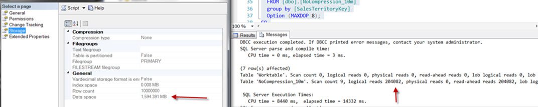
/**Message Results:
Table ‘test10m’. Scan count 9, logical reads 204082, physical reads 0, read-ahead reads 204082, lob logical reads 0, lob physical reads 0, lob read-ahead reads 0.
SQL Server Execution Times:
CPU time = 8016 ms, elapsed time = 14522 ms.**/
Since each logical read represents one 8 KB page then the formula for calculating the total amount of data returned by the query is the following:
Logical Reads x 8 (single DB page) / 1024 (MB)
204,082 x 8 / 1024 = 1,594 MB
Since there are no indexes on the table, this calculation can be double checked by simply looking the size of the data in the table.
While there is a lot more involved with perforamnce tuning a SQL Server data warehouse server to meet end user requirements, server throughput (MB/seconds) and query size (MB) represent two of the most important factors.