
While Finance may be a complex and multifaceted industry, the core goal of any financial institute is very straightforward: to detect and mitigate risks while maximizing profit. This objective is easy to summarize, however it is certainly no small feat to attain!

The ever-expanding role of technology in the Finance sector poses several risks to consumers, which directly affect an organization’s reputation. Furthermore, as the reach of innovative technology expands, so too does market size. According to IBIS, market size (as measured by revenue) is slated to increase by 4.4% in 2021 as a result of more per capita disposable income. Unfortunately, these growth increases are accompanied by risk increases; more clients with more perceived expendable income can result in higher loan risks. Essentially, financial institutes are burdened with the dichotomy of having to mitigate risks to customers, while also mitigating customer risks to themselves.
To combat these challenges, many financial agencies are turning to Machine Learning. Machine Learning is a branch of Artificial Intelligence (AI) in which computer algorithms improve and “learn” automatically through training data. These models can then be applied to new data to make predictions or decisions relevant for the business.
In our last Financial risk mitigation post, we demonstrated how Machine Learning can tackle alleviating risks to customers by using classification methods to detect fraudulent charges. In this blog, we’ll address the benefit of financial companies protecting themselves from potentially risky customers by applying Machine Learning methods to loan applications. To demonstrate the benefits of Machine Learning in loan risk analysis, we’ll walk through the process of building a simple Gradient Boosting Tree (GBT) model within Azure Databricks.
Preparing the Data
This notebook uses a public dataset from Lending Club comprised of 2,260,701 funded loans from 2012 through 2017. Each of these loans include information provided by applicants, as well as the current loan status and latest payment information as shown in the Databricks screenshot below:
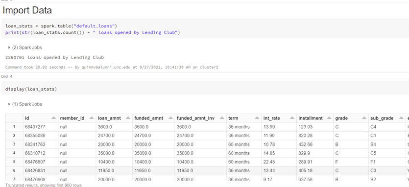
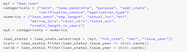
Once we have the data loaded into the notebook, we can perform data cleansing (i.e. handling null values, converting columns to appropriate formats, etc.) and feature engineering (the process of creating new, potentially insightful variables based off existing ones). Since the objective is to predict which loans will most likely default, we need to create a target prediction label.
This column, named bad_loan, is produced by encoding paid-off loans as 0 and defaulted loans as 1. Creating a net amount column (total_payments – loan_amount) will also be beneficial for evaluating the solution’s overall business value. In this model, we are analyzing only loans classified as closed.
Exploring the Data
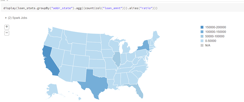
With the preprocessing phase complete, we can move into data exploration to acquire a better understanding of the data’s distribution and relationships. As we might expect, we can see in the map below that there are higher loan counts among the more populous states.
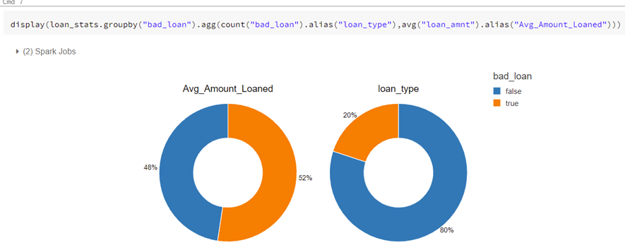
We can also see that bad loans account for 20% of our cases; however, their loan amount on average is nearly identical to paid-off loans.
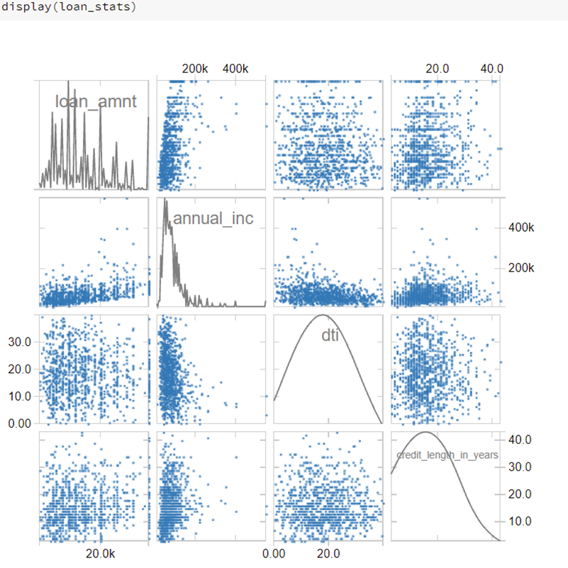
Examining distributions of individual variables, as well as possible correlations is also beneficial for the modeling process. Despite GBT’s ability to handle multi-collinearity in predictions, removing highly linearly correlated variables could improve statistical inferences including feature importance. Below is a scatter plot of several of the numerical dependent variables. It appears that annual income is skewed more to the right than the other variables, and that significant relationships do not exist.
Building, Training, and Testing the Model
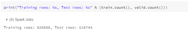
With this knowledge of our dataset, we are now ready to build, train, and test a model. We start by labeling our independent and dependent variables, and splitting our data into a training and validation set. This technique allows us to see how well our model performs with data it has yet to encounter.
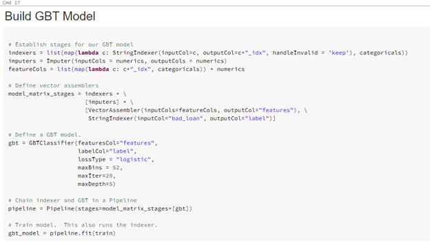
Next, we construct an input vector based off our labeled variables and a GBT classifier with hardcoded parameters based on data size. Using a pipeline, we then execute these stages on the training data set.
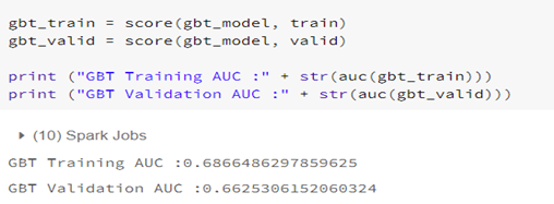
We can evaluate model performance through the Area Under the Curve (auc) score, where 100% indicates a perfect model. For both the training and validation sets, the score we’ve achieved is approximately 70%. This is a decently performing model, considering that for simplicity’s sake, only one parameter set was tested. In a standard practice, we would use parameter grid search plus cross-validation techniques to train the model for the most optimal parameters.
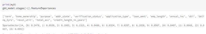
In addition to obtaining accurate predictions, knowing the model’s highest contributing features can aid in driving business decisions. In our model, the term of the loan and the state are the most significant features.
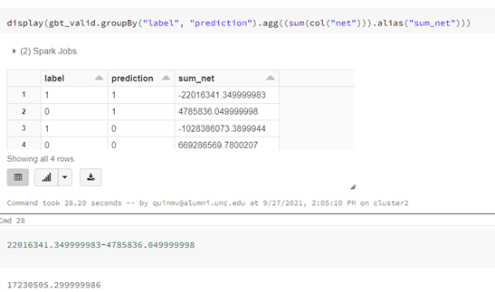
Finally, we can evaluate if the main objective of decreasing a company’s loan risk was achieved. By combining the confusion matrix with the created net column, we can calculate a monetary value of the model. In this case, the model saved approximately $22 million by correctly labeling a bad loan. Even correcting for approximately $5 million in false positives, the overall net value of the model is $17 million.
Overall, Machine Learning is an excellent resource for navigating the tough financial sector. It can not only assist companies in better serving their clients, but also prevents companies from investing in risky scenarios.
More Information
3Cloud offers a variety of resources to help you learn how you can leverage Machine Learning in your sector. Please contact us directly to see how we can help you explore your about modern data analytics options and accelerate your business value.