For the past few months, we’ve been helping a global Financial Services company with their ongoing Snowflake implementation, which will ultimately sunset older, on-premises data marts in Oracle and SQL Server. Part of this engagement has included Power BI QuickStarts, where we’ve gotten to roll up our sleeves and put Power BI to work on top of Snowflake warehouses. As we partnered with the client’s various technology teams, we quickly realized that success lay less in implementing additional features into their environment, than in working to correct several modeling assumptions they were making within Power BI.
Inspired by ideas presented in Microsoft and Snowflake’s joint webinar, and actual issues encountered during our client’s QuickStarts, this post will aim to educate on how to create efficient Power BI solutions on top of Snowflake.
 Connecting to Snowflake
The first step to building Power BI solutions on top of Snowflake is to connect to a Snowflake warehouse. This post assumes you already know how to use the native Snowflake connector in Power BI to connect to a warehouse. If this is a new concept, Microsoft’s documentation has an easy-to-follow tutorial on how to establish a connection from Power BI Desktop.
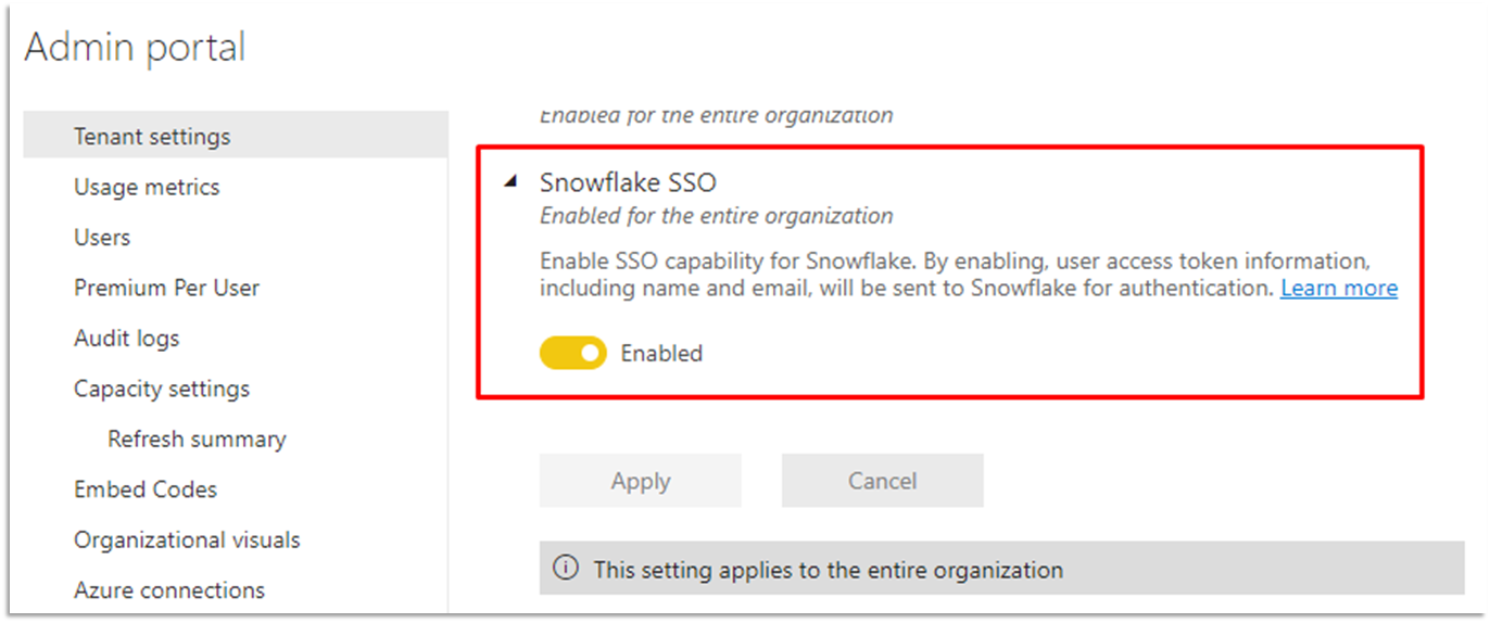
Power BI also supports SSO access to Snowflake. While the topic of Snowflake SSO is out-of-scope for this post, this Snowflake documentation has a thorough walkthrough on the process end-to-end. For Power BI Administrators, there is a tenant setting you need to be aware of, and enable, if looking to leverage Snowflake SSO.
Power BI Dataset Connectivity Modes
When working with Snowflake, or any relational source system, it’s important to understand what your options are for building semantic models on top of it in Power BI. Below, we’ll introduce the three different types of dataset connectivity modes in Power BI and provide general considerations for each.
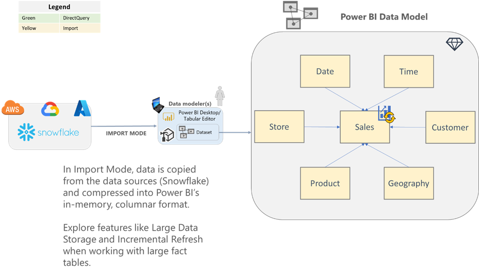
Import
Import mode is the most common mode we see when working with customers. With import mode, you ingest a copy of the source data into an in-memory dataset. Power BI’s underlying storage engine (VertiPaq/xVelocity) provides significant compression capabilities. A quick rule of thumb is that you can typically expect about 10x compression when importing data into Power BI. That said, there are several variables that can affect compression, which we’ll talk more about below.
| Import Mode | |
| Pros | Cons |
| Typically, the fastest report and query performance due to the data being stored in-memory within Power BI. | Data latency could be an issue since this is a cache of the source data. Use scheduled refreshes to keep your dataset current. |
| Full Power BI feature set is available. | Large source data will need thoughtful up-front planning. Features like Power BI premium Large Dataset Storage and Incremental Refresh should be considered for importing large data volumes. |
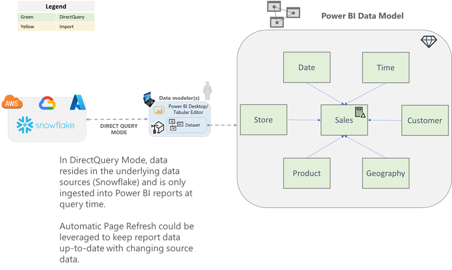
Direct Query
With DirectQuery datasets, no data is imported into Power BI. Instead, your Power BI dataset is simply metadata (e.g., tables, relationships) of how your model is structured to query the data source. Data is only brought into Power BI reports and dashboards at query-time (e.g., a user runs a report, or changes filters).
| DirectQuery Mode | |
| Pros | Cons |
| Dataset size limits do not apply as all data still resides in the underlying database. | Typically, query-time performance will suffer, even when querying a cloud data warehouse like Snowflake. |
| Datasets do not require a scheduled refresh as data is only retrieved at query-time. | Concurrency (e.g., multiple users running reports) against DirectQuery datasets could cause performance issues against the underlying database. |
| Near real-time reports can be developed by leveraging automatic page refresh and Power BI Premium. | Limited Power Query and data modeling feature set. |
Here’s a good reference for a thorough list of considerations when using DirectQuery mode.
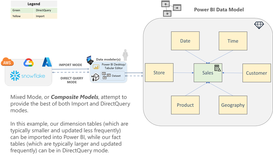
Composite
Composite models attempt to combine the best aspects from Import and DirectQuery modes into a single dataset. With Composite models, data modelers can configure the storage mode for each table in the model. A common design pattern for working with large, frequently-updated fact tables is to set the central fact table as DirectQuery mode, and set the surrounding dimension tables as Import or dual mode. This pattern allows your contextual data points (dimension attributes), that are used for filtering and slicing-and-dicing, to be stored in memory.
Common Mistakes
Direct Query all the Things!
The first common mistake we encountered in our QuickStarts was that developers only used, or wanted to use, DirectQuery mode. While DirectQuery mode isn’t inherently bad, it should only be explored if you have specific requirements that make it a necessity. For example, extremely large data volumes, frequently changing data, or the need for Snowflake SSO, are all candidates for DirectQuery.
BFTs
The next most common mistake we encountered in our customers’ datasets was what I call BFTs, or Big Fat/Flat Tables. While it may be easy to get started with a BFT model (after all, it’s only a single table), you will quickly realize the importance of a well-defined data model. We always recommend dimensional models/ Star Schemas for our customers because the benefits far outweigh the initial data shaping it will take to create one. We outline reasons you should use a star schema model in the Power BI Optimization Best Practices section below.
Speaking of dimensional models, that brings us to our next common mistake…
Bidirectional Relationships Galore!
One technology team we partnered with had a great star schema design implemented in Snowflake. However, once that design was imported into Power BI, they broke it with bidirectional relationships. Because they were leveraging bidirectional relationships between each table, they were unable to model a constellation schema (multiple facts) because they kept running into the dreaded “ambiguity” errors. This happens when the tabular engine has multiple paths, or directions, it can take to filter a table within the model, but no clear instruction on which one, so rather than guess, it doesn’t evaluate at all. Since the relational model was already comprised of one-to-many relationships between dimensions and facts, simply changing all the relationships to a “single” filter direction allowed them to consolidate several Power BI datasets into one. This dataset consolidation then allowed them to easily analyze different business processes by their conformed dimensions within the same reports.
Size of Data > Number of Records
This mistake refers to a common statement we heard throughout our QuickStarts:
“We want to stress test Power BI with n million rows.”
These customer statements inevitably led to the typical consultant response:
“Well, that depends on…”
The number of records you can import into Power BI depends on several variables, including:
- How wide (number of columns) is your table?
- What is the cardinality (number of distinct values) for each column?
- What is the data type of each column?
- What is the data length of each column?
A quick example was when we were importing investment metrics into Power BI. The source table had 100 columns, of which, 85 were numeric ratios with a precision of 12 decimal places. Simply rounding those 85 metrics down to four decimal places decreased the cardinality of those columns, thus increasing how well Power BI could compress the data in memory. The net result was the size of our overall memory footprint of the dataset being cut in half. There is more on data size in the Power BI Optimization Best Practices section below.
Power BI Optimization Best Practices
This section highlights key Power BI data modeling best practices. Many of the best practices listed also appear in the Build Scalable BI Solutions Using Power BI and Snowflake webinar mentioned in the Introduction. Additionally, we’ve added a few best practices from our own experience. Lastly, all the best practices listed can be applied to other relational database sources, too! These aren’t exclusive to connecting to Snowflake.
Dimensional Models
As mentioned above, we always recommend taking the time to properly model your data into a star schema design. There are several reasons for this, including:
- Cleaner and easier to use than a BFT – Related attributes and measures can be stored in the same tables for quick navigation
- The granularity (level of detail) of a BFT may not properly reflect the business model, resulting in workarounds, poor calculations, and limits to scenarios which can be performed
- Instead, creating separate fact tables for each subject area or business process, then relating them with conformed dimensions will allow you to analyze metrics from different business processes by the dimensions they share
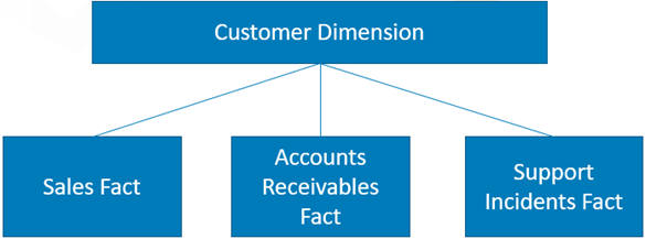
1- e.g., Analyzing sales, support incident requests, and delinquent accounts receivables all for a single customer
- You may find significant memory savings by separating your contextual information out into dimensions, then storing only integer surrogate keys in your fact tables

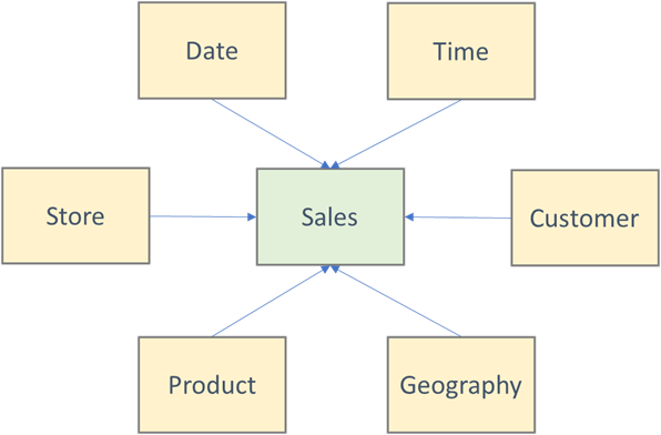
2 – Simple star schema with a centralized fact table
Limit Number of Visuals
Each visual on a report page will generate its own DAX query (yes, even slicers). When using DirectQuery mode, these DAX queries also get translated to SQL and executed against the underlying Snowflake database. For these reasons, it’s imperative to be thoughtful with the design of each report page. You should strive to limit the number of visuals on a page, not only for performance, but also in the name of conveying information at a glance.
Limit Interactivity between Visuals
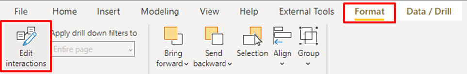
When building report pages, you should also consider the interactivity (e.g., cross-filter, cross-highlight) between your visuals. This is especially true for reports that are developed on top of a DirectQuery dataset or table. The reason is that every time you click a data point in a visual, if interactivity is enabled, it will attempt to filter or highlight the other visuals on your page, thus kicking off another round of queries. You can manually set the interactivity between visuals by selecting Edit Interactions from the Format pane, then toggling how each visual interacts with other visuals on the page.
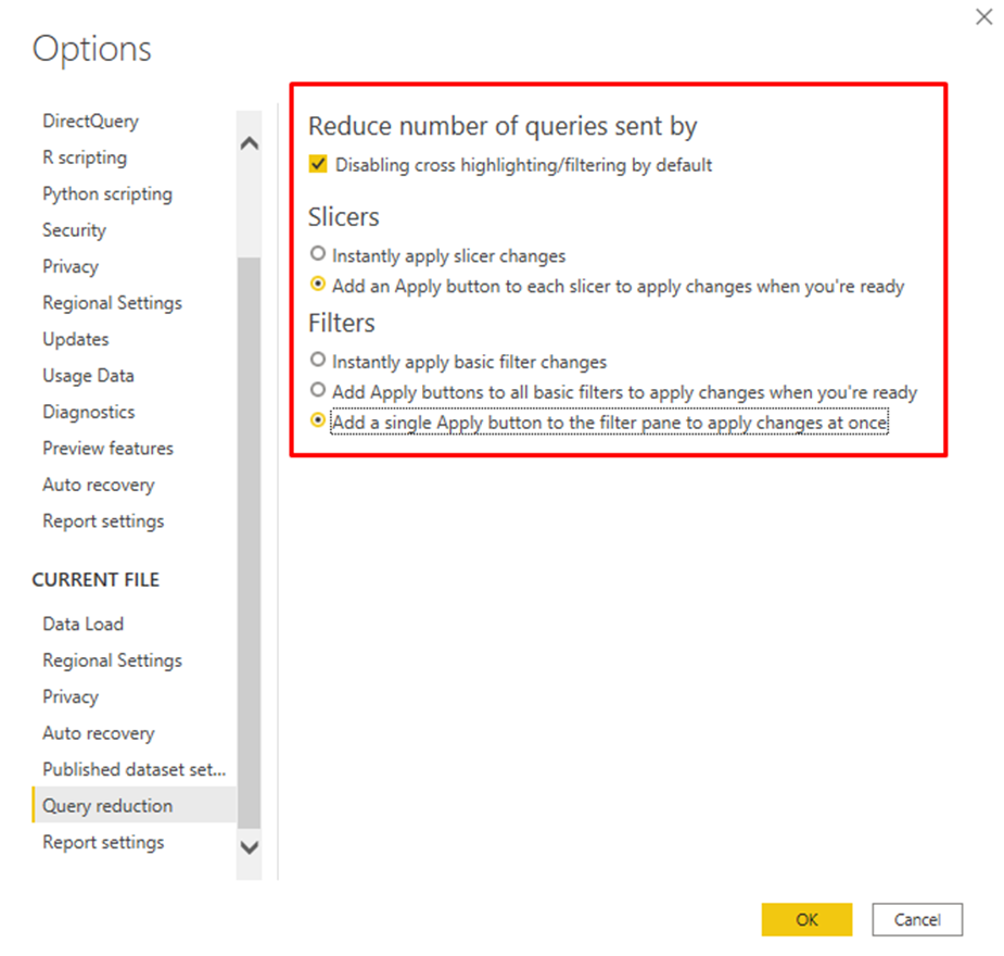
Query Reduction
If you want a quicker way to eliminate all interactivity by default, then check out Query Reduction. Query Reduction is a report-level feature that allows report creators to reduce the number of queries that get generated by interactivity and filtering actions (e.g., slicers and filter pane).
Query Reduction can be accessed from:
File –> Options and Settings –> Options –> Current File –> Query Reduction
Query Reduction allows you to:
- Disable cross highlighting/filtering by default
- Add an Apply button to each slicer, so you can control when filtering occurs
- Add an Apply button to each filter, or the entire filter pane, so you can control when filtering occurs
Patrick at Guy in a Cube has a great video on Query Reduction and how it can help performance in your DirectQuery reports.
Assume Referential Integrity
The Assume Referential Integrity button is an advanced feature found in the relationships dialog. This button only appears when modifying a relationship in a DirectQuery model. This feature will tell Power BI to generate inner joins instead of outer joins when generating the SQL that executes in Snowflake. If you are confident in the data quality of your Snowflake tables, then enabling this feature will allow Power BI to generate more efficient SQL queries to retrieve data.
Only use Bidirectional Filters when Necessary
This is a common mistake that we see customers who are new to tabular modeling make all the time. 99% of the time you should stick with a single filter direction in your table relationships. This means that the filter should only flow from the one side (dimension) to the many side (fact) within the model.
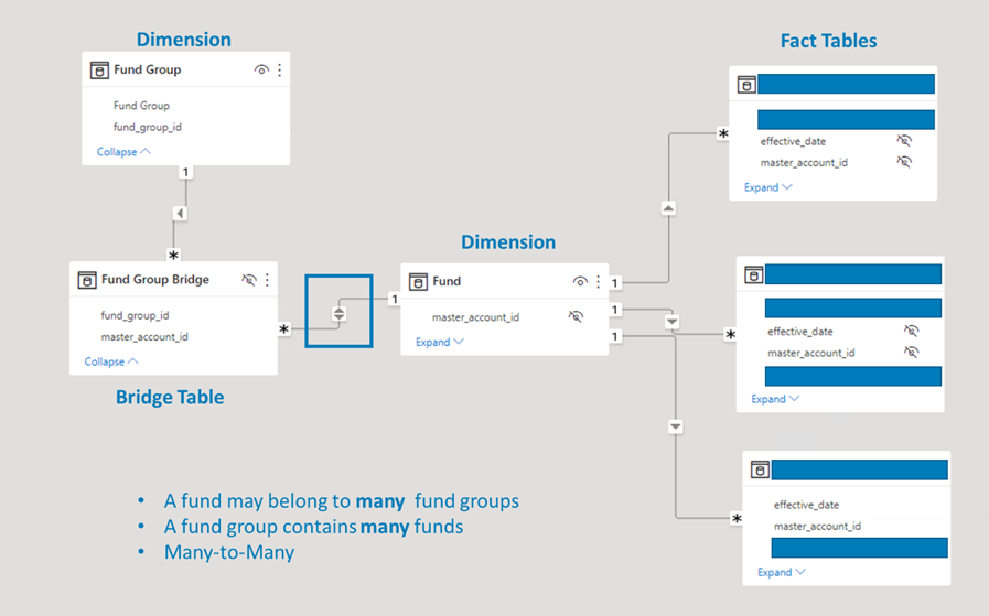
However, rather than say “never use bidirectional relationships”, we think it’s important to call out acceptable use cases. The primary use case involves modeling many-to-many relationships. Take the screenshot below for example. Our customer wanted to group different investment funds:
- A fund can belong to more than one fund group
- A fund group can contain more than one fund
To solve this problem, we created a traditional factless fact/bridge table to establish the set of keys. The bridge table allows you to create one-to-many relationships between the two dimensions back to the bridge table. The bidirectional relationship comes into play when we want to allow filter, slicer, or grouping capabilities by fund groups. We need the filter to flow from the bridge table to the main fund dimension that is connected to all our downstream facts. Without the bidirectional relationship, our fund groups would filter our bridge table, but nothing else.
Only Bring in Data that’s Needed for Analysis
This is probably the simplest best practice on this list, yet often one of the most violated. It is very common to see customers pull in things like:
- Fact table keys
- Business/natural keys
- GUIDs that aren’t used in relationships
- ETL/auditing metadata fields
Common examples like the list above should remain in your data sources if they aren’t providing any analytical value. In addition to limiting the fields that are brought into your model, you should also consider if there are any ways to filter the data that you bring into your model. The best models are the simplest ones that provide only the data points you need for analysis.
Aggregations
Aggregations are a set of Power BI features that allow data modelers and dataset owners to improve query performance over large DirectQuery datasets. Currently, there are two types of aggregations in Power BI: User-Defined Aggregations and Automatic Aggregations.
The premise for both types of aggregations is to boost report performance by reducing the number of “round trips” queries must take to return results to a report. The obvious caveat to aggregations is that it may introduce a level of data latency to your queries if data is being imported into memory, as is the case with Automatic aggregations. In this case, if a report query can be satisfied by an aggregation, then it will not be querying the data source directly. Aggregations should be explored if you want to improve query-time performance, without fully sacrificing the need for DirectQuery operations.
Incremental Refresh
Incremental refresh is an important feature to consider when working with large tables that you would like to import into memory. With Incremental Refresh, partitions are automatically created on your Power BI table based on the amount of history to retain, as well as the partition size you would like to set. Since data modelers can define the size of each partition, refreshes will be faster, more reliable, and able to build history over time.
When setting up Incremental Refresh, keep in mind the following:
- You must create RangeStart and RangeEnd date/time parameters. These parameters must be set to a date/time data type and must be named RangeStart and RangeEnd.
- The initial refresh in the Power BI service will take the longest due to the creation of partitions and loading of historical data. Subsequent refreshes will only process the latest partition(s) based on how the feature was configured.
- Using Incremental Refresh within a dataset in Premium capacity will allow additional extensibility via the XMLA endpoint. For example, SQL Server Management Studio (SSMS) can be used to manage partitions.
In Summary
Developing efficient Power BI solutions on top of Snowflake doesn’t need to be a daunting task. Rather, it needs thoughtful requirements gathering to ensure the optimal Power BI features are being leveraged for the desired use case. In the case of our customer, educating them on common Power BI modeling mistakes and more effective alternatives, opened a door of opportunities that they didn’t think were possible a few months ago.
Our team of BI experts can help you learn more about Power BI and how to use it effectively in your organization. Contact 3Cloud today.