Become the Maestro of your Genomics Workflow with Bioconductor and Microsoft R Server

Microsoft R Server is an enterprise-class tool for hosting and managing parallel and distributed workloads of R processes on servers. Organizations that need to process large amounts of data or perform complex processing on the data benefit the most from a parallel architecture like Microsoft R Server. It uses the RevoScaleR package, which makes parallelization easy.

In genomics research, we often interact with large amounts of data from complex pipelines in a diverse array of formats. Luckily, Bioconductor helps make this process simpler by packaging up common sets of processes in ready-to-use R code.

Harnessing the power of both Bioconductor and Microsoft R Server together can help streamline the processing of your genomics data.

All About Bioconductor

Bioconductor is an open-source, open-development software project to provide tools for the analysis and comprehension of high-throughput genomic data. It is based primarily on the R programming language. In other words, it’s an extension of R that is specialized for bioinformatics and genomics analyses.

Installation

Once R (either base R or Microsoft R Server) is installed on your local machine, installing Bioconductor is simple. Open R and use the following commands to grab the latest version of Bioconductor.

Once the biocLite script has loaded, you can now call any desired packages.

Now you are ready to use over 1,000 Bioconductor packages!

Workflows

The field of genomics is very broad, but Bioconductor will often have a solution for every area. The Bioconductor site is rich with workflow examples to help connect the dots for your research. Check out Bioconductor’s help section for a list of the available workflows.

Here are a few of my favorites:

• Sequence Analysis – Import fasta, fastq, BAM, gff, bed, wig, and other sequence formats. Trim, transform, align, and manipulate sequences. Perform quality assessment, ChIP-seq, differential expression, RNA-seq, and other workflows.
• Variant Annotation – Read and write VCF files. Identify structural location of variants and compute amino acid coding changes for non-synonymous variants and predict consequence of amino acid coding changes.
• High Throughput Assays – Import, transform, edit, analyze and visualize flow cytometric, mass spec, HTqPCR, cell-based, and other assays.
• Transcription Factor Binding – Find candidate binding sites for known transcription factors via sequence matching.
• Cancer Genomics – Download, process, and prepare TCGA, ENCODE, and Roadmap data to interrogate the epigenome of cultured cancer cell lines as well as normal and tumor tissues with high genomic resolution.

Package Database

Didn’t see a workflow that exactly fit your needs? No problem! Bioconductor has a nice list of available packages that will help you find the right one for the problem at hand. Using the search box shown below, I searched for the term “eQTL” (Expression Quantitative Trait Loci) to find packages related to that topic.

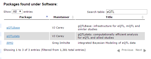
For more information, you can check out the package list here.

Enhancing your Workflow with Microsoft R Server

Whether you are using the pre-made workflows or ended up creating your own, you can likely speed up processing time by running your Bioconductor/R scripts in parallel. Microsoft R Server and RevoScaleR make this easy.

Let’s take the Annotating Genomic Variants workflow, for example.

.vcf files are often very large and sometimes difficult to process or summarize due to their size. Using the VariantAnnotation::locateVariants function from Bioconductor makes this process more automated. We can use this function to identify where a variant falls with respect to gene structure, e.g., exon, utr, splice site, etc. We use the gene model from the TxDb.Hsapiens.UCSC.hg19.knownGene package loaded earlier.

## Use the 'region' argument to define the region
## of interest. See ?locateVariants for details.
cds <- locateVariants(vcf, txdb, CodingVariants())
five <- locateVariants(vcf, txdb, FiveUTRVariants())
splice <- locateVariants(vcf, txdb, SpliceSiteVariants())
intron <- locateVariants(vcf, txdb, IntronVariants())

all <- locateVariants(vcf, txdb, AllVariants())

If we want to start summarizing the variants, we could use sapply to repetitively perform some operation over the entire data object. Take a look at the highlighted lines below.

aa <- predictCoding(vcf, txdb, Hsapiens)
idx <- sapply(split(mcols(aa)$QUERYID, mcols(aa)$GENEID, drop=TRUE), unique)
sapply(idx, length)

## Summarize variant location by gene:
sapply(names(idx), 
    function(nm) {
        d <- all[mcols(all)$GENEID %in% nm, c("QUERYID", "LOCATION")]
        table(mcols(d)$LOCATION[duplicated(d) == FALSE])
    })

##            125144 162514 23729 51393 7442 84690
## spliceSite      0      2     0     0    1     0
## intron          0      0     0     0    0     0
## fiveUTR         0      2     0     1    3     5
## threeUTR        0     25     2     1    2     0
## coding          0      5     0     3    8     0
## intergenic      0      0     0     0    0     0
## promoter        1     23     0     0   15    11

This code easily summarizes the .vcf file in a few seconds. However, the NA06985_17.vcf.gz file is only a small (35MB) sample from human Chromosome 17. What if you were to use multiple files to assess a sample population such as the ones available from 1000 Genomes? sapply might take a while…

We can use the RevoScaleR package to parallelize the summarization function in the code. By using rxExec to distribute the processing over multiple cores of a processor or even multiple nodes on a Hadoop cluster, we can speed up the processing time tremendously. In the sample code below, we use the rxExec function to split up the processing by GeneID.

## Summarize variant location by gene using rxExec from Microsoft R Server:
vcflocationsummary <- function(nm) {
        d <- all[mcols(all)$GENEID %in% nm, c("QUERYID", "LOCATION")]
        table(mcols(d)$LOCATION[duplicated(d) == FALSE])
    }
rxExec(vcflocationsummary, rxElemArg(GENEID))

 Note: this is only sample code. To fully use this workflow, visit Bioconductor’s workflow variants.

Try it Out

Now that we have explored how easy it is to speed up your genomics workflows using Microsoft R Server, you can try it out for yourself. Pick a workflow that fits your needs and then use it. Once you start seeing where the processing bottlenecks are, think about using RevoScaleR‘s parallelization functions to speed things up. Look for loops and apply functions as prime candidates for distributed processing.

First time using Microsoft R Server and the RevoScaleR? Microsoft’s documentation is a great place to start. To compare the RevoScaleR functions, read Explore R and RevoScaleR in 25 functions. If you still have questions, please reach out to us and we will be happy to help!